Excel is an effective and versatile tool for managing and analyzing large datasets. However, encountering errors during data processing is unavoidable. This is where the IFERROR function in Excel becomes invaluable.

The IFERROR function helps display a custom message when a formula results in an error.

In this article, we will delve into the following topics in depth:

Now, let's examine each of these topics in turn!

Download the Excel Workbook to practice and learn how to utilize the IFERROR function in Excel –

download excel workbookIFERROR-Function-in-Excel.xlsx

Introduction

The IFERROR function in Excel enables you to specify a value to return if a formula results in an error. If your calculation produces errors such as #N/A, #VALUE!, #REF!, #DIV/0!, #NUM!, #NAME?, you can manage these errors using the IFERROR function, which allows you to replace the error with a 0, a blank cell, or a custom message.

The syntax of the IFERROR function in Excel is as follows:

=IFERROR(value,value_if_error)

• value – The formula you wish to evaluate.
• value_if_error – The value to be shown if the evaluated formula results in an error.

If the formula's result is not an error, the function will simply display the formula's result.

Types of Errors

Here are the various types of errors you might encounter while working in Excel:

• #REF! – This error appears when a cell referenced in a formula does not exist or is invalid.
• #VALUE! – Excel shows an #VALUE! error when the variable used in the formula is of an unsupported type.
• #DIV/0! – This error occurs when attempting to divide a number by zero, a value equivalent to zero, or a blank cell.
• #NULL! – This error is displayed when the range specified in the formula is invalid and you have used an incorrect character instead of the required one.
• #SPILL! – When a formula cannot populate all the cells it should, the first cell where the formula is entered shows the #SPILL! error.
• #NAME? – This error occurs due to a spelling mistake in the formula name, cell range, or named range, or when text is entered without quotes.
• #NUM! – This error indicates that the values in formulas are invalid and the calculation cannot be performed due to limitations or errors.

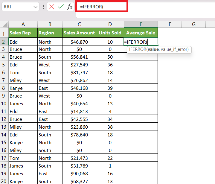
Example 1 – Handling Division Errors

In this example, we need to calculate the average sale per record by dividing the total sales amount by the units sold. However, dividing 0 by 0 will result in an error.

Thus, we need to manage division by zero errors effectively.

STEP 1: Input the IFERROR function into an empty cell.

=IFERROR(

STEP 2: Enter the first argument – value. Here, you first need to input the formula to calculate the average sale.

=IFERROR(C2/D2,

STEP 3: Enter the second argument – value_if_error. In this case, we want to display “0” if there is an error.

=IFERROR(C2/D2,0)

Apply the same formula to the remaining cells by dragging the lower right corner downwards.

Now you have all the results!

Example 2 – Dealing with Missing Data

IFERROR can be used to notify the user when the searched value is absent from the dataset. Instead of displaying an error, the function can show a message such as “Not found”.

Let’s consider an example of this scenario.

STEP 1: Here, we are using the VLOOKUP function to find the Date of Joining for the employee ID listed in cell G1 within the dataset.

=VLOOKUP(G1,A2:D32,4,0)

• G1 is the value we want to look up (Employee ID 1000).
• A2:D32 indicates the entire source data table.
• 4 specifies that we want to retrieve the date of joining, which is in the fourth column.
• 0 ensures an exact match.

You will see a #N/A error! This happens because 1000 is not present in the source table. Let's improve its appearance with IFERROR!

STEP 2: By enclosing the VLOOKUP formula within IFERROR, we can replace this error with a specific message, like “Not Found”:

=IFERROR(VLOOKUP(G1,A2:D32,4,0), “Not Found”)

With this adjustment, your result is now clean and free of errors!

The IFERROR function in Excel is a powerful tool for handling errors and improving user experience. It is versatile and essential for anyone working with data and formulas in Excel.

Click here to learn about the Top 20 Common Excel Errors you might encounter, and how to address them.

The above is the detailed content of 2 Useful Examples of IFERROR Function in Excel – A Beginner’s Guide. For more information, please follow other related articles on the PHP Chinese website!