Mastering the art of custom number formatting in Microsoft Excel is crucial for presenting data with precision and clarity. This guide delves into Excel's capabilities for customizing number, date, and text displays, ensuring your data communicates effectively and maintains a professional appearance.

Key Takeaways

• Custom Number Format: Excel offers detailed customization options for displaying numbers, text, dates, and times, enhancing presentations with features like text annotations or displaying figures in millions.
• Placeholders and Symbols: Using placeholders (#, 0) and symbols ($, %) provides flexible data presentation options.
• Formatting Techniques: Excel supports both basic (comma separation) and advanced (scientific notation) formatting to enhance readability.
• Date and Time Formats: Custom formats allow for precise temporal data display, aiding in understanding timelines and schedules.
• Efficiency: Mastering shortcuts and applying custom formats across datasets increases Excel productivity and analytical efficiency.

Table of Contents

Introduction to Excel Custom Formatting

The Importance of Precision in Data Presentation

When dealing with data in Excel, presenting numbers accurately and clearly is vital for effective communication. Precision in data presentation not only improves readability but also ensures that your audience understands the data's significance without being overwhelmed by numbers.

Overview of Excel’s Custom Format Options

Excel offers a wide range of formatting options that go beyond the standard formats. While the built-in "Number," "Currency," and "Date" formats meet most needs, sometimes data requires a more customized approach. Custom format options allow you to define how Excel displays text, numbers, dates, and times with precision and style tailored to your specific needs.

For example, you might want to display figures in millions, add commas, or include text annotations within a cell without altering the data's integrity. Excel's Custom Number Formatting feature is a powerful tool in your data presentation toolkit.

Mastering the Basics of Custom Number Formats

Understanding Placeholders and Symbols

Exploring Excel's custom number formats, you'll encounter various placeholders and symbols, each with a specific function. The # (pound sign) and 0 (zero) are essential for number display. The # acts as a flexible placeholder, adjusting to the presence or absence of a digit. In contrast, 0 ensures a display, filling in with zeros if the number is too short.

For instance, the format 0.00 will display a half (0.5) as 0.50, ensuring two decimal places are always visible. Changing this to #.00 still shows .50, but without the leading zero. This difference allows for both consistency and flexibility in presenting numerical data.

Additionally, Excel provides special characters like $ for currency, % for percentages, and @ for text manipulation. When used effectively, these tools can help you present numbers with both precision and creativity.

Applying Basic Custom Formats for Numbers and Text

Understanding the fundamental custom formats in Excel can significantly enhance the presentation of your spreadsheets. For numbers, applying a comma can neatly separate thousands, and a decimal point can set the precision for digits following the decimal.

For example, the format #,##0.00 will transform 12345.6 into 12,345.60, incorporating commas for thousands and ensuring two decimal places.

If you're dealing with currency, simply prepend the currency symbol, like $, to make the value as clear as possible: $#,##0.00.

Text can also be formatted easily. Use the @ symbol in your custom format to incorporate text within a numeric format. If you want to add a unit of measure, such as kg, to a number, your format might look like 0 "kg", turning 50 into 50 kg.

These basic elements of custom formatting enable you to give your data a professional and polished appearance, aiding in both its understanding and impact.

Advanced Techniques in Custom Numerical Formats

Showcasing Scientific Notation and Large Numbers

When dealing with extremely small or large numbers, Excel's scientific notation is invaluable. It allows for compact representation of numbers using a base and an exponent, where the E in Excel's notation stands for "Exponent." Here are a couple of custom format variations:

• The 0.00E 00 format transforms 1500500 into 1.50E 06. It controls the significant figures and positions of the exponent.

• A slight modification to #0.0E 0 results in 1.5E 6, slightly less precise but still in scientific notation.

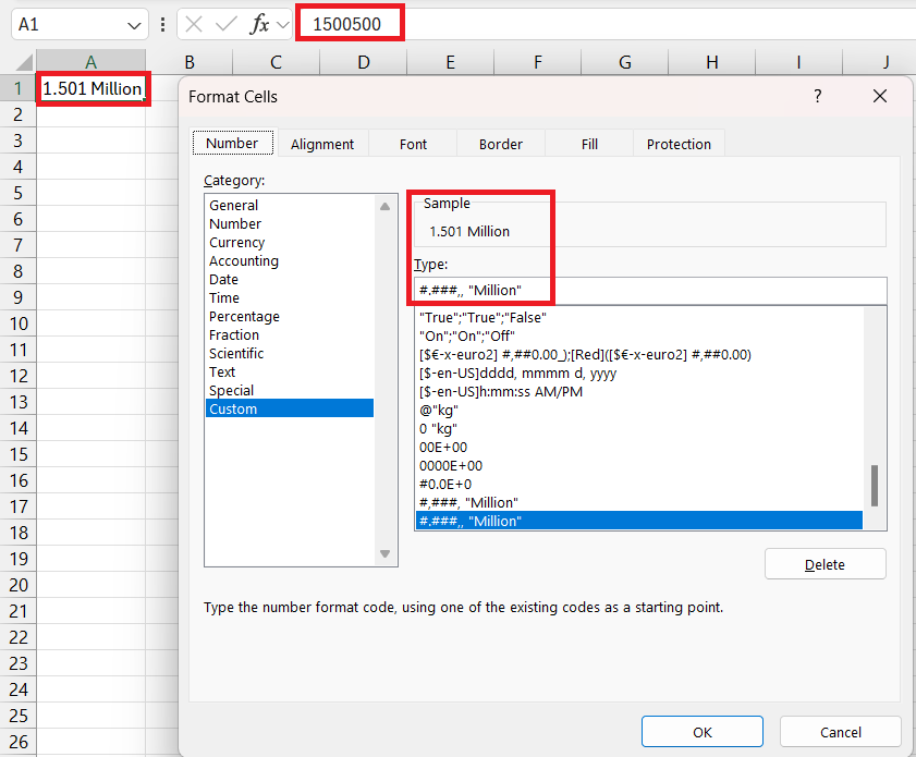
For dealing with large magnitudes like millions and billions, custom formats allow you to abbreviate the numbers. For instance, a custom format like #.###,, "Million" displays 1,500,500 as 1.501 Million. This approach is not only easier on the eyes but also simplifies reading and understanding financial and statistical data.

Excel also offers the flexibility to highlight these figures in different colors, depending on their value or context, which we'll explore later.

Displaying Negative Values and Zeroes Creatively

Excel's capabilities extend into the realm of aesthetics when displaying negative values and zeros. You can format these distinctively using custom formats.

Negative Numbers: You may want a red font for clarity or parentheses for an accounting look. Here's how to add flair to negative values:

0.00;[Red](0.00) This format displays positive numbers with two decimal places, while negative numbers appear in red within parentheses, highlighting them immediately.

These creative options allow you to subtly inform viewers about the nature of your data without altering a single digit.

Tailoring Date and Time Formats to Your Needs

Extracting More from Excel’s Date and Time Capabilities

Excel's date and time formatting capabilities are robust, allowing you to display temporal data in virtually any way needed. Beyond the standard date and time formats, you can tailor custom formats to meet specific reporting requirements or personal preferences.

For dates, Excel's custom formats allow you to include or omit elements such as the day of the week, the month as a number or text, and the year in two or four digits. For example, you can transform '4/1/2018' to 'Sunday, April 1, 2018', by using the custom format code dddd,mmmm d, yyyy.

Time can be formatted to show hours, minutes, and seconds in various notations. Whether you need the 24-hour format or prefer the AM/PM distinction, custom formats have you covered. For instance, a format like hh:mm:ss AM/PM will display '23:59:00' as '11:59:00 PM'.

Leveraging these date and time capabilities to their fullest potential means more intuitive data, where every cell pinpoints the exact moment in time you're trying to communicate. This can be especially useful for project timelines, appointment schedules, and historical data analysis among other applications.

Custom Strategies for Managing Temporal Data

Managing temporal data in Excel requires a thoughtful approach to custom formatting, especially when the default date and time settings don't quite align with your needs. Excel's date/time serial number system can work to your advantage once you understand how to tap into it.

Consider a scenario where you'd like to separately display the date and time from a timestamp. Using custom formats like mm/dd/yyyy and hh:mm AM/PM each in their dedicated column, can split your timestamp into its components for clearer analysis.

If you need to track just workdays or exclude holidays from your reports, you could employ the WORKDAY function alongside these custom formats for operational schedules and deadline tracking.

To highlight durations rather than points in time, employ [hh]:mm:ss AM/PM for time lengths that exceed 24 hours, ensuring you get a true reflection of time elapsed, be it for project tracking or event duration studies.

Incorporating these custom strategies for managing temporal data ensures you're not just recording time but interpreting it in ways that benefit the decision-making process.

Utilizing Colors and Conditions in Formatting

Visually Distinguish Data with Conditional Color Coding

Color coding adds a layer of intuition to your data, helping to quickly distinguish between varying data points based on conditional logic. Excel custom formats allow you to assign different colors to numbers, text, and even background fills to emphasize or de-emphasize certain values.

Let's explore this through an example. Suppose you want to highlight passing grades in green and failing grades in red. You'd use a custom format like this:

[>=10][Green]”P(pán)ass”;[When applied, any grade 10 or above in a cell is boldly marked as “Pass” in green, while anything below 10 is starkly labeled as “Fail” in red. These visual cues enable a quicker comprehension of the data at a glance, perfect for dashboards and reports where speed is of the essence.

Additionally, this use of condition-based coloring is adaptable and can be extended beyond grades to financial thresholds, inventory levels, or anything where clear demarcation of data is beneficial.

Leveraging Custom Formats for Data Analysis

Custom formats in Excel aren't just about making data look good—they are fundamental for efficient data analysis. By incorporating data-appropriate custom formats, you ensure accurate representation, making interpretation both intuitive and precise.

For instance, consider visualizing financial statements where variance from a budget is crucial. With custom formats, positive variances can show in blue, indicating surplus, while negative figures appear in red, clearly marked as a deficit. A custom format like this might look like 0.00;[Red]-0.00;[Blue]0.00, where each color represents a different financial status.

Another prime example of leveraging custom formats is the use of in-cell bars (conditional formatting) that serve as mini-charts, where the length and color of the bar within the cell can quickly depict relative values without the need for a separate chart.

Leveraging these analytical capabilities enhances the interpretative power of your data, allowing patterns and insights to surface rapidly, ultimately aiding in more informed decision-making.

Tips and Tricks for Excel Formatting Proficiency

Shortcut Methods for Common Formatting Scenarios

Efficiency in Excel often hinges on knowing the right shortcuts to navigate common tasks quickly. When you're immersed in data and time is critical, being familiar with keyboard shortcuts for number formats can save you valuable time. Here's a quick guide to shortcut methods for common formatting scenarios:

• To apply the General format, press Ctrl Shift ~.
• For Currency format, use Ctrl Shift $.
• If you need the Percentage format, Ctrl Shift % is your combo.
• To switch to Scientific format, Ctrl Shift ^ does the trick.
• For the Date format, it's Ctrl Shift #.
• And to set the Time format, press Ctrl Shift @.

Remembering these shortcuts can significantly speed up your formatting work, allowing you to quickly adapt cell appearance for clearer data presentation.

Real-World Examples to Guide Your Practice

Crafting Telephone Numbers and Financial Figures

When faced with untidy lists of numbers in a spreadsheet, you might want to bring some order, particularly with telephone numbers and financial figures that need to meet standardized formats. Custom formats come to the rescue by letting you impose a consistent structure across your dataset.

Crafting Telephone Numbers: To ensure telephone numbers are easily readable, you'll often want to insert spaces, parentheses, and hyphens.

Managing and Streamlining Your Custom Formats

Editing and Deleting Custom Formats Effectively

Navigating the world of Excel's custom formats involves not just creating them but also knowing how to edit or retire them when they're no longer applicable. If you need to make changes to a custom number format, remember that Excel doesn't exactly allow "editing" in the traditional sense. Instead, when you alter an existing format, you're essentially creating a new one that will then appear in your workbook's Custom Category list.

Should you need to delete a custom number format, follow these steps:

STEP 1: On the Home tab, go to the Number group and click More Number Formats at the bottom of the number format list.

STEP 2: In the Format Cells dialog box, click Custom.

STEP 3: From the list, select the unwanted custom number format and hit the Delete button.

Two key reminders for this process:

• Built-in formats are unremovable, indicated by the Delete button being greyed out.
• Once a custom format is deleted, it's gone for good; if you need it again, you'll have to recreate it from scratch.

Remember to regularly audit your custom formats, deleting any that have outlived their usefulness to keep your workbook streamlined and efficient.

Organizing and Applying Formats Across Multiple Datasets

Efficiently managing and applying custom formats across multiple datasets can greatly enhance your productivity in Excel. By organizing your custom number formats, you create a consistency that not only makes your data more readable but also eases the application of these formats across various datasets within your workbook or even across different workbooks.

Start by creating a library of your most frequently used custom formats. To do this, define and apply them in one worksheet, and they'll be stored under the 'Custom' category within the 'Format Cells' dialogue box. Once there, these formats are ready for reuse without the need to redefine them each time.

When working across multiple datasets, especially if they span various worksheets or workbooks, use the 'Format Painter' tool. This handy feature allows you to quickly copy a cell's format and apply it to other cells, even if they're in different workbooks.

For workplace efficiency, consider sharing your custom format library with colleagues by using template workbooks. This ensures that when your team works on related projects, everyone is using the same standardized formats, enhancing collaboration and communication.

Keep in mind that while custom number formats are stored within Excel's workbook where they were created, the cell formats can be transferred between workbooks using copy-paste actions, ensuring uniformity in all of your shared data.

FAQs on Excel Custom Formatting

How Do I Create a Custom Number Format from Scratch?

Creating a custom number format from scratch in Excel is straightforward. Select the cell or range of cells you want to format, and then press Ctrl 1 or right-click and choose Format Cells. In the dialog box, select the 'Custom' category. Here you can enter your desired format using the code structure provided. For example, 0.00 will format your number to two decimal places. Click 'OK' to apply your custom format. Remember, this adds the format to your workbook's library for future use.

Can I Apply Custom Number Formats to Charts or Graphs?

Yes, you can apply custom number formats to charts or graphs in Excel. Right-click the data labels or axis labels on your chart and select 'Format Axis' or 'Format Data Labels. Navigate to the 'Number' tab and input your custom number format into the 'Format Code' box. Your custom formats will help clarify the data presented in your charts for better insight.

What Are the Limitations of Excel’s Custom Formats?

While Excel's custom formats are versatile, they do have limitations. Custom formats affect only how data looks, not the actual data itself, so calculations remain unaffected. Also, there's a maximum format code length of 255 characters, and custom formats do not change a cell's underlying data type. Plus, Excel may not retain these formats if your worksheet is exported to a different software program.

Are Custom Formats Saved When I Share an Excel File?

Yes, custom formats are saved with the Excel file. So, when you share an Excel file, the recipient will see your custom formats without needing to reapply them. However, ensure that the recipient uses the same version of Excel for compatibility and that they don't open the file in a different program that might not recognize custom Excel formatting.

How do I custom number format M and K in Excel?

To format numbers in thousands (K) or millions (M), you can create a custom format. Select your cells, press Ctrl 1, and go to 'Custom'. For thousands, use #,"K". This will show 12,000 as 12K. For millions, use #,,"M". This turns 1,200,000 into 1.2M. The comma indicates the scaling factor, reducing the number of displayed digits while adding the respective letter. Apply and press 'OK'.

The above is the detailed content of Custom Number Format in Excel – Fast Number Formatting Guide. For more information, please follow other related articles on the PHP Chinese website!