Color-coding in Microsoft Excel isn't just about enhancing visual appeal; it's a potent tool for swiftly navigating through intricate datasets. By implementing color-coded systems, you can accelerate data analysis, easily identifying patterns and insights. This guide will delve into techniques for counting and summing by color in Excel.

Key Takeaways:

• Enhanced Navigation: Color coding facilitates quicker data review, transforming numerical rows into visual indicators for trends and patterns.
• Conditional Formatting: Make use of Excel’s built-in features to boost visual appeal and streamline data analysis.
• Manual Methods: Learn to use the SUBTOTAL function effectively to sum by color, utilizing Excel’s filtering features.
• Simple Formulas: Use basic Excel formulas such as SUMIF for an uncomplicated approach to summing by color.
• Advanced Techniques: Delve into VBA macros for a more dynamic and customizable method of summing by color, enhancing your Excel skills.

Table of Contents

Introduction to Color-Coded Summing in Excel

The Importance of Color-Coding in Data Analysis

Color coding in Excel goes beyond mere aesthetics; it's a practical method for rapidly navigating through complex datasets. Envision sifting through rows of data to uncover insights; colors serve as visual markers, significantly hastening the process.

In the realm of data analysis, this color-coded approach is particularly effective for categorizing items or emphasizing key performance indicators—each color denoting a different data point or category, making it simple to spot patterns and trends.

Setting Up Your Excel Sheet for Summing by Color

Preparing your data to provide quick insights using conditional formatting is straightforward. Begin by selecting the cells you wish to format, then navigate to the ‘Home’ tab. Select ‘Conditional Formatting’ and choose from the various rules available.

Whether you're coloring cells based on their values, creating data bars, or setting up color scales, Excel provides ample options. This not only improves the visual appeal but can significantly cut down the time spent searching for outliers or patterns within your dataset.

Manual Methods to Sum by Color in Excel

Utilizing the SUBTOTAL Function with Filtered Colors

For summing by color, the SUBTOTAL function in Excel is incredibly useful, as it only considers visible rows in a filtered list.

STEP 1: First, filter your data by color—select your data, go to the ‘Data’ tab, and click ‘Filter’.

STEP 2: Then, choose ‘Filter by Color’ and select the color you're focusing on.

STEP 3: After filtering, add a blank row at the bottom of your dataset; this is where you'll enter your SUBTOTAL formula.

STEP 4: Enter =SUBTOTAL(9, range) where ‘range’ is the cells you want to sum.

This will give you the sum by color.

Remember, using ‘9’ as the function number ensures you're summing only the cells that aren't hidden by the filter. Use 2 as a function number to count the filtered cells.

Summing Cells by Color with Basic Excel Formulas

If you prefer not to use advanced methods, basic Excel formulas can still achieve the desired result. Since Excel doesn't have a built-in function for summing by color, you'll need a workaround. Use the color to set a condition, assign a value to that condition—perhaps “1” for colored cells and “0” for non-colored.

Use the SUMIF function to add up the cells that meet your criterion.

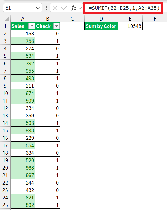
While this doesn't directly sum by color, it provides a simpler alternative for those less familiar with VBA or add-ins.

Advanced Techniques for Color-Coded Summation

Creating VBA Macros for Dynamic Summing by Color

Harness the power of customization with VBA macros to make summing by color effortless.

STEP 1: Press Alt F11 to access the Visual Basic for Applications (VBA) editor.

STEP 2: Go to ‘Insert’ and select ‘Module’ to open a new module window.

STEP 3: Enter the following macro:

Function SumByColor(CellColor As Range, SumRange As Range) As Double

Dim Sum As Double

Dim MyCell As Range

Sum = 0

‘ Check each cell in the sum range

For Each MyCell In SumRange

If MyCell.Interior.Color = CellColor.Interior.Color Then

Sum = Sum MyCell.Value

End If

Next MyCell

SumByColor = Sum

End Function

Once you've created and saved the function, you can use it in your Excel workbook like any other function.

If you have a cell (let’s say I1) with the color you want to sum, and a range of cells (B2:BG5) where some cells match the color of I1, you can use the function in another cell like this:

=SumByColor(I1,B2:G5)

This formula will return the sum of all cells in the range B2:G5 that have the same background color as the cell I1.

Tips and Best Practices for Summing by Color in Excel

Ensuring Precision in Color-Based Calculations

Ensuring precision in your color-based calculations is essential, as even minor errors can distort your data analysis. Be mindful that functions or add-ins used for summing by color might not automatically update when cell colors change.

To prevent this, manually refresh your formulas or check the add-in settings for auto-update options. It's also advisable to periodically verify your totals with a manual count, particularly after altering your dataset's color scheme.

Keeping Data Current for Real-time Summation

To keep your data analysis up-to-date, maintaining real-time summation is crucial. This involves setting up a system where changes in cell values or colors are immediately reflected in your sum totals. Regularly use functions and tools that automatically recalculate with each change. Explore the settings of your Excel add-ins to ensure they're configured for automatic recalculation.

If you're using macros, strategically place buttons to quickly re-run them. By doing so, your color-coded sums remain as dynamic as the datasets they represent, enabling you to make informed decisions promptly.

FAQs on Excel Color-Coded Summing

How can I activate color-coded summing in Excel?

To activate color-coded summing in Excel, apply conditional formatting to your dataset to highlight cells of interest. Then, use functions like SUBTOTAL to sum only visible cells after filtering by color. For more dynamic summing, consider writing a VBA macro or using a specialized Excel add-in that directly supports this feature.

What are the constraints of using color as a criterion for summing?

The primary constraint of using color as a criterion for summing in Excel is that it doesn't inherently consider cell color, and there's no direct function for this task. Sums based on color require manual methods, VBA scripts, or third-party add-ins. Additionally, these methods may not automatically update when cell colors change, except when using filters with the SUBTOTAL function.

Can I sum by color without using macros?

Yes, you can sum by color without macros by using Excel’s ‘Filter by Color’ feature and then applying the SUBTOTAL function to sum the visible cells in that color.

How do I calculate the total of colored cells in Excel?

You can calculate the total of colored cells in Excel by using its ‘Filter by Color’ feature and then applying the SUBTOTAL function to sum the visible cells in that color. Alternatively, you might use an add-in like Ablebits’ Ultimate Suite, which simplifies the process with its ‘Count & Sum by Color’ tool, eliminating the need for complex functions or manual counting.

What is conditional formatting in Excel?

Conditional formatting in Excel is a feature that allows you to apply specific formatting to cells that meet certain criteria. You can use it to highlight, color-code, add data bars, color scales, or icon sets to your data based on its value. This dynamic tool aids in visualizing data, identifying trends, and distinguishing outliers at a glance.

The above is the detailed content of Excel Tips: How to Count and Sum by Color in Excel Effortlessly. For more information, please follow other related articles on the PHP Chinese website!