


Use the ampersand (&) or CONCATENATE to combine data first by entering a formula like =A1 & " " & B1 in a new cell, then paste as values to preserve all data before merging. 2. Use Merge Across or Merge Cells only after combining data to avoid losing content from cells other than the top-left one. 3. For multiple rows, use a helper column with a formula such as =A1 & ", " & A2 & ", " & A3 to consolidate data before merging. 4. Alternatively, use "Center Across Selection" by selecting cells, pressing Ctrl 1, going to Alignment, choosing Center Across Selection to achieve a merged appearance without actual merging or data loss. Always back up data, never use "Merge & Center" on cells with multiple values, combine data first with formulas, and use visual formatting afterward to safely retain all information.
Merging cells in Excel while keeping all your data isn't as straightforward as it seems—because when you use the standard "Merge & Center" button, Excel only keeps the data from the top-left cell and discards the rest. But there are simple ways to merge cells without losing any information. Here’s how.

1. Use the Ampersand (&) or CONCATENATE to Combine Data First
Before merging cells visually, combine the contents of the cells into one using a formula.
Example:
Say you have:

- A1: "John"
- B1: "Doe"
You want to merge them into one cell as "John Doe".
Enter this formula in a new cell (like C1):

=A1 & " " & B1
Or use:
=CONCATENATE(A1, " ", B1)
This combines the text with a space in between. Once the data is combined, you can:
- Copy the result
- Right-click the target cell → Paste Values (to remove the formula)
- Then safely merge the cells visually if needed
This method preserves all your original data and gives you full control over formatting.
2. Use the Merge Across or Manual Merge (After Combining Data)
Once your data is combined into a single cell using the method above, you can merge cells for visual formatting:
- Select the cells you want to merge (e.g., A1:B1)
- Go to the Home tab
- Click the small arrow in the Merge & Center group
- Choose Merge Across or Merge Cells
? Important: Only do this after combining the data—otherwise, you’ll lose everything except the top-left value.
3. Use a Helper Column to Combine Multiple Rows
If you're merging multiple rows (e.g., A1, A2, A3), you can stack the data first:
In a blank column (say B1), use:
=A1 & ", " & A2 & ", " & A3
Then copy the result, paste as values, and merge the original cells for layout purposes.
4. Alternative: Use "Center Across Selection" (Best for Display Only)
If you just want the appearance of merged cells without actually merging (and risking data loss), try this:
- Select the cells you'd normally merge (e.g., A1:C1)
- Press Ctrl 1 to open Format Cells
- Go to the Alignment tab
- Under Horizontal, choose Center Across Selection
- Click OK
? This makes the label look centered across the range without merging cells or losing data. Great for headers!
Key Tips:
- Always backup your data before merging
- Never use "Merge & Center" on multiple cells with data unless you’re okay with losing everything except the top-left value
- Combine data first with formulas, then format visually
- Use "Center Across Selection" when you only need the visual effect
Basically, Excel doesn’t let you merge cells with data safely by default—so you have to combine the content before merging. Do that, and you’ll avoid losing any important info.
The above is the detailed content of How to merge cells in Excel without losing data?. For more information, please follow other related articles on the PHP Chinese website!

Hot AI Tools

Undress AI Tool
Undress images for free

Undresser.AI Undress
AI-powered app for creating realistic nude photos

AI Clothes Remover
Online AI tool for removing clothes from photos.

Clothoff.io
AI clothes remover

Video Face Swap
Swap faces in any video effortlessly with our completely free AI face swap tool!

Hot Article
Hot Tools

Notepad++7.3.1
Easy-to-use and free code editor

SublimeText3 Chinese version
Chinese version, very easy to use

Zend Studio 13.0.1
Powerful PHP integrated development environment

Dreamweaver CS6
Visual web development tools

SublimeText3 Mac version
God-level code editing software (SublimeText3)
Hot Topics


 What should I do if the frame line disappears when printing in Excel?
Mar 21, 2024 am 09:50 AM
What should I do if the frame line disappears when printing in Excel?
Mar 21, 2024 am 09:50 AM
If when opening a file that needs to be printed, we will find that the table frame line has disappeared for some reason in the print preview. When encountering such a situation, we must deal with it in time. If this also appears in your print file If you have questions like this, then join the editor to learn the following course: What should I do if the frame line disappears when printing a table in Excel? 1. Open a file that needs to be printed, as shown in the figure below. 2. Select all required content areas, as shown in the figure below. 3. Right-click the mouse and select the "Format Cells" option, as shown in the figure below. 4. Click the “Border” option at the top of the window, as shown in the figure below. 5. Select the thin solid line pattern in the line style on the left, as shown in the figure below. 6. Select "Outer Border"
 How to filter more than 3 keywords at the same time in excel
Mar 21, 2024 pm 03:16 PM
How to filter more than 3 keywords at the same time in excel
Mar 21, 2024 pm 03:16 PM
Excel is often used to process data in daily office work, and it is often necessary to use the "filter" function. When we choose to perform "filtering" in Excel, we can only filter up to two conditions for the same column. So, do you know how to filter more than 3 keywords at the same time in Excel? Next, let me demonstrate it to you. The first method is to gradually add the conditions to the filter. If you want to filter out three qualifying details at the same time, you first need to filter out one of them step by step. At the beginning, you can first filter out employees with the surname "Wang" based on the conditions. Then click [OK], and then check [Add current selection to filter] in the filter results. The steps are as follows. Similarly, perform filtering separately again
 How to change excel table compatibility mode to normal mode
Mar 20, 2024 pm 08:01 PM
How to change excel table compatibility mode to normal mode
Mar 20, 2024 pm 08:01 PM
In our daily work and study, we copy Excel files from others, open them to add content or re-edit them, and then save them. Sometimes a compatibility check dialog box will appear, which is very troublesome. I don’t know Excel software. , can it be changed to normal mode? So below, the editor will bring you detailed steps to solve this problem, let us learn together. Finally, be sure to remember to save it. 1. Open a worksheet and display an additional compatibility mode in the name of the worksheet, as shown in the figure. 2. In this worksheet, after modifying the content and saving it, the dialog box of the compatibility checker always pops up. It is very troublesome to see this page, as shown in the figure. 3. Click the Office button, click Save As, and then
 Where to set excel reading mode
Mar 21, 2024 am 08:40 AM
Where to set excel reading mode
Mar 21, 2024 am 08:40 AM
In the study of software, we are accustomed to using excel, not only because it is convenient, but also because it can meet a variety of formats needed in actual work, and excel is very flexible to use, and there is a mode that is convenient for reading. Today I brought For everyone: where to set the excel reading mode. 1. Turn on the computer, then open the Excel application and find the target data. 2. There are two ways to set the reading mode in Excel. The first one: In Excel, there are a large number of convenient processing methods distributed in the Excel layout. In the lower right corner of Excel, there is a shortcut to set the reading mode. Find the pattern of the cross mark and click it to enter the reading mode. There is a small three-dimensional mark on the right side of the cross mark.
 How to set superscript in excel
Mar 20, 2024 pm 04:30 PM
How to set superscript in excel
Mar 20, 2024 pm 04:30 PM
When processing data, sometimes we encounter data that contains various symbols such as multiples, temperatures, etc. Do you know how to set superscripts in Excel? When we use Excel to process data, if we do not set superscripts, it will make it more troublesome to enter a lot of our data. Today, the editor will bring you the specific setting method of excel superscript. 1. First, let us open the Microsoft Office Excel document on the desktop and select the text that needs to be modified into superscript, as shown in the figure. 2. Then, right-click and select the "Format Cells" option in the menu that appears after clicking, as shown in the figure. 3. Next, in the “Format Cells” dialog box that pops up automatically
 How to use the iif function in excel
Mar 20, 2024 pm 06:10 PM
How to use the iif function in excel
Mar 20, 2024 pm 06:10 PM
Most users use Excel to process table data. In fact, Excel also has a VBA program. Apart from experts, not many users have used this function. The iif function is often used when writing in VBA. It is actually the same as if The functions of the functions are similar. Let me introduce to you the usage of the iif function. There are iif functions in SQL statements and VBA code in Excel. The iif function is similar to the IF function in the excel worksheet. It performs true and false value judgment and returns different results based on the logically calculated true and false values. IF function usage is (condition, yes, no). IF statement and IIF function in VBA. The former IF statement is a control statement that can execute different statements according to conditions. The latter
 How to merge cells in WPS table
Mar 21, 2024 am 09:00 AM
How to merge cells in WPS table
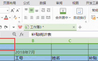
Mar 21, 2024 am 09:00 AM
When we use WPS to make our own tables, the header of the table needs to be in a cell. At this time, the question arises, how does WPS merge cells? In this issue, I have brought you the specific operation steps, which are below. Please study them carefully! 1. First, open the WPS EXCEL file on your computer. You can see that the current first line of text is in cell A1 (as shown in the red circle in the figure). 2. Then, if you need to merge the words "Subsidy Statistics Table" into the entire row from A1 to D1, use the mouse to select cell A1 and then drag the mouse to select cell D1. You can see that all cells from A1 to D1 have been selected (as shown in the red circle in the figure). 3. Select A
 How to insert excel icons into PPT slides
Mar 26, 2024 pm 05:40 PM
How to insert excel icons into PPT slides
Mar 26, 2024 pm 05:40 PM
1. Open the PPT and turn the page to the page where you need to insert the excel icon. Click the Insert tab. 2. Click [Object]. 3. The following dialog box will pop up. 4. Click [Create from file] and click [Browse]. 5. Select the excel table to be inserted. 6. Click OK and the following page will pop up. 7. Check [Show as icon]. 8. Click OK.
